Section 9.3: Regression

1. Identify the sample residuals / errors
   \[e = y - \widehat{y} = y - (b_{0} + b_{1} x)\] from a regression of \(y\) on \(x\) (aka from predicting a response \(y\) using a predictor \(x\)).
2. Describe and interpret a residual plot of \(e\) versus \(x\) or equivalently of \(e\) versus \(\widehat{y}\).

Section 9.4: Variation and Prediction Intervals

1. Give two equivalent definitions of the coefficient of determination, aka \(R^{2}\), aka R-sq.
2. State the common (though erroneous) way to use \(R^{2}\) as a way to evaluate a simple linear regression model.
3. Relate the coefficient of determination to the sample linear correlation coefficient \(r_{xy}\).

Chapter 9 (Additional Handout): Assumptions, Diagnostics, and Inferences for the Simple Linear Regression Model with Normal Errors

Link to Handout

1. Identify the five main assumptions of the simple linear regression model with normal residuals.
2. Explain what the above assumptions indicate about how the true errors / residuals \(\epsilon_{i}\) should look when the simple linear regression model with normal residuals is appropriate.
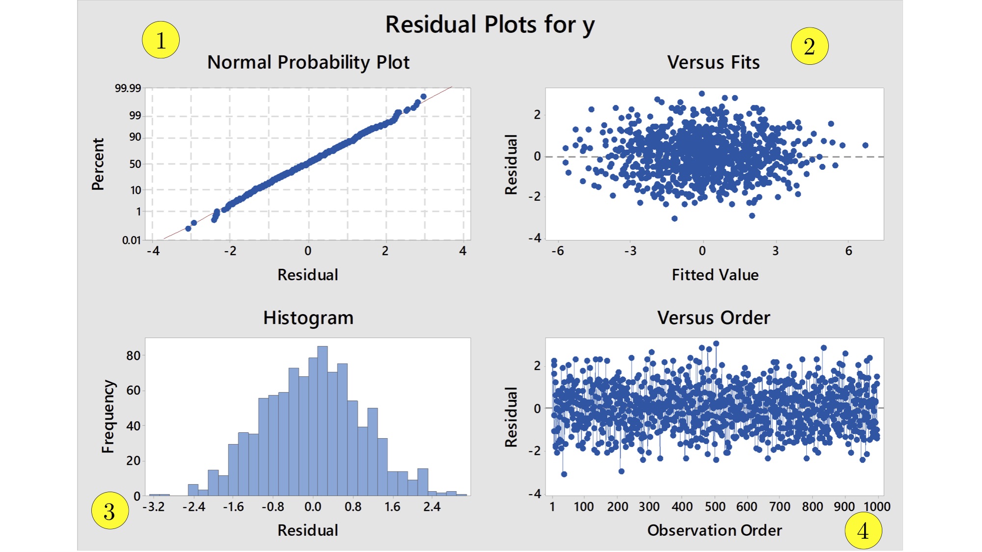
3. Use the diagnostic plots generated by Minitab, like the ones below, to determine whether the simple linear regression model with normal residuals is appropriate for the paired data under consideration.
   
4. Interpret the standard errors for the estimators \(b_{0}\) and \(b_{1}\) reported by Minitab in terms of margins of error. Minitab calls the standard errors SE Coef.
5. Identify the hypothesis tests associated with the \(P\)-values reported by Minitab.
6. Interpret the P-values reported by Minitab in terms of hypothesis tests for the population intercept \(\beta_{0}\) and slope \(\beta_{1}\).