POSTS
Salvaging Lost Significance via Randomization: Randomized \(P\)-values for Discrete Test Statistics
Last time, we saw that when performing a hypothesis test with a discrete test statistic, we will typically lose size unless we happen to be very lucky and have the significance level \(\alpha\) exactly match one of our possible \(P\)-values. In this post, I will introduce a randomized hypothesis test that will regain the size we lost. Unlike a lot of randomization in statistics, the randomization here comes at the end: we randomize the \(P\)-value in order to recover the size. In many cases (ideally!), experimentalists use randomization at the beginning of their experiment, by (ideally) randomly sampling from a population and then randomly assigning units to a treatment. But the extra step of randomizing at the end, when they’re eagerly awaiting to find out whether they’ve been so-blessed with significance stars, they may balk at randomization, even though it makes their test more powerful. I will allow them their balking (I might, too, if my career depended on accumulating many, many stickers), and in the next post I will discuss a method that gets rid of the random element of randomized \(P\)-values while still guarding against the conservativeness of the test.
For this exercise, let’s consider a right-sided test. (Why? Because I had already made all the figures and schematics for a right-sided test before writing the last post, and don’t want to remake them for the left-sided test!) Again, consider the case of performing a hypothesis test \[\begin{aligned} H_{0} &: p \leq p_{0} \\ H_{1} &: p > p_{0}\end{aligned}\] for a binomial proportion \(p\) using a binomial random variable \(X \sim \mathrm{Binom}(n, p)\). The classical right-sided \(P\)-value is then \[P = P_{p_{0}}(X \geq x_{\mathrm{obs}}).\] We know that this will, generally, be slightly too small at a boundary value of \(x_{\mathrm{obs}}\): the difference between the largest \(P\)-value less than or equal to \(\alpha\) and \(\alpha\) will be non-zero unless we happen to have a “nice” sample size where that \(P\)-value is close to \(\alpha\). But we also know that \(P_{p_{0}}(X > x_{\mathrm{obs}})\) will be slightly too big, since this is the first \(P\)-value that is stricly greater than \(\alpha\). The idea of a randomized \(P\)-value is to add a little fuzz to the classical right-sided \(P\)-value that will place us somewhere between \(P_{p_{0}}(X \geq x_{\mathrm{obs}})\) and \(P_{p_{0}}(X > x_{\mathrm{obs}})\). That is, the randomized \(P\)-value is \[P_{\mathrm{rand}} = P_{p_{0}}(X > x_{\mathrm{obs}}) + U \times P_{p_{0}}(X = x_{\mathrm{obs}})\] where \(U\) is a uniform random variable on \((0, 1)\) that is independent of \(X\).
Why does this work? Consider the sketch below, which shows the survival function \(S(k) = P(X > k)\) and its left-continuous analog \(S(k^{-}) = P(X \geq k)\):
n <- 10
p <- 0.5

alpha = 0.4

ns <- 0:n

Ss <- pbinom(ns, n, p, lower.tail = FALSE)

par(mar=c(5,5,2,1), cex.lab = 2, cex.axis = 2)
plot(ns, Ss, type = 's',
     xlab = expression(italic(k)), ylab = 'Probability')

Ss.p1 <- Ss + dbinom(ns, n, p)
points(ns, Ss, col = 'blue', pch = 16)
lines(ns, Ss.p1, col = 'red', type = 'p', pch = 16)

abline(h = alpha, lty = 3, col = 'purple')
abline(h = c(0, 1), lty = 3)
abline(v = c(0, n), lty = 3)

legend('topright', legend = c(expression(P(italic(X) >= italic(k))),
                              expression(P(italic(X) > italic(k)))),
       col = c('red', 'blue'), pch = 1, cex = 1.2)

arrows(0.5, 0, 0.5, alpha, code = 3, col = 'purple', lwd = 2, length = 0.15)
text(x = 0.5, y = alpha+0.05, labels = expression(alpha), col = 'purple', cex = 2)
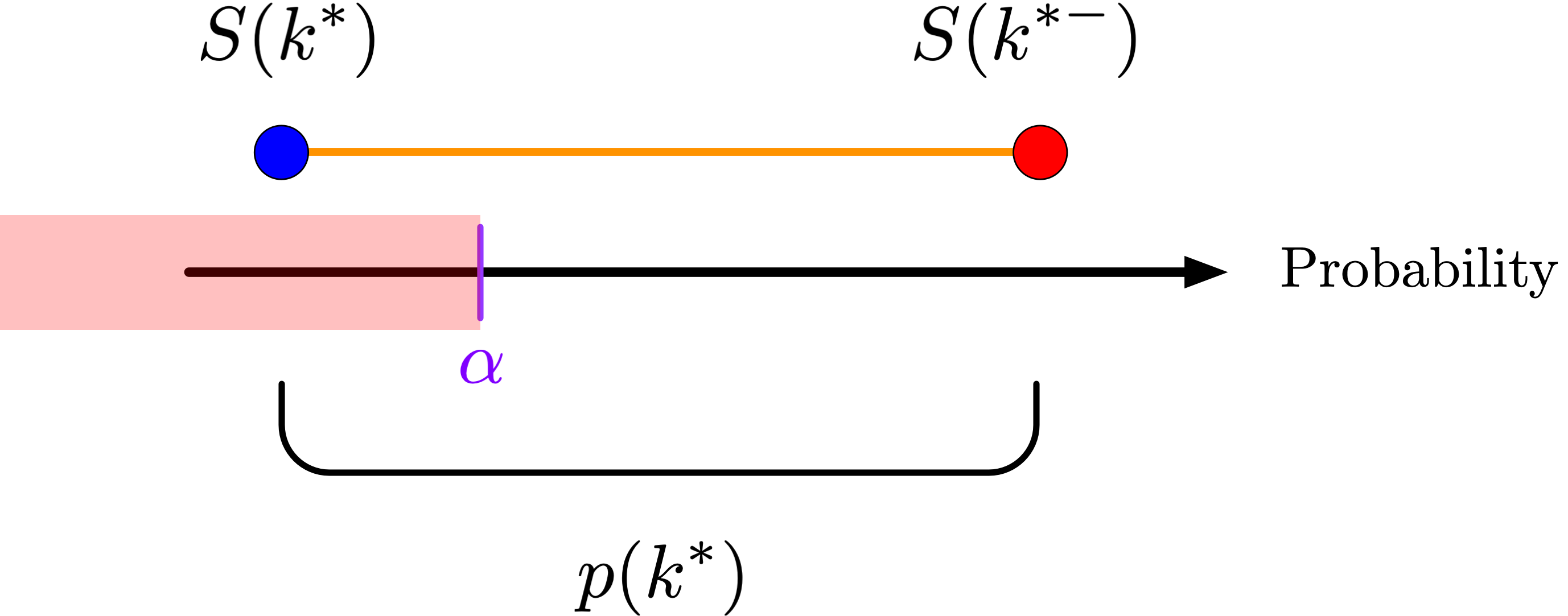
and we should only reject when the \(P\)-value falls at or below \(\alpha\). Because \(U\) is uniform, the probability that this occurs is \[P\left(U \leq \frac{\alpha - S(k^{*})}{p(k^{*})} \right) = \frac{\alpha - S(k^{*})}{p(k^{*})}.\] So on the boundary of the rejection region, we reject \(H_{0}\) with probability \(\frac{\alpha - S(k^{*})}{p(k^{*})}\). Let \(\phi(X)\) be our rejection rule, i.e. the function that is 1 when we reject the null hypothesis and 0 otherwise. Then \(\phi\) is a random function with the conditional distribution \[P(\phi(X) = 1 \mid X = k) = \begin{cases} 0 &: k < k^{*} \\ \frac{\alpha - S(k^{*})}{p(k^{*})} &: k = k^{*} \\ 1 &: k > k^{*} \end{cases}.\] Given this definition, it’s straightforward to prove that the probability that we reject the null hypothesis, that is, that \(\phi(X) = 1\), is in fact \(\alpha\): \[\begin{aligned} P(\phi(X) = 1) &= \sum_{k} P(\phi(X) = 1 \mid X = k) P(X = k) \\ &= \sum_{\{k : k < k^{*}\}} 0 \cdot p(k) + \frac{\alpha - S(k^{*})}{p(k^{*})} p(k^{*}) + \sum_{\{k : k > k^{*}\}} 1 \cdot p(k) \\ &= \alpha - S(k^{*}) + S(k^{*}) \\ &= \alpha,\end{aligned}\] just as we wanted.
So a little uncertainty at the end buys us back our size, and we attain the desired significance level.