POSTS
How Confident Are We that Masks "Work"? Confidence Functions and the DANMASK-19 Study
Attention Conservation Notice: I use a recent study about COVID-19 as an excuse to demo an R package I am developing. Some other reasons not to read this: (a) I am not an epidemiologist and (b) I do not plan to explain confidence functions enough for the uninitiated to make sense of this post.
Andrew Gelman had an interesting post recently about the DANMASK-19 trial out of Denmark. This study randomized individuals to recieve a mask recommendation and a supply of 50 surgical masks (or not):
Encouragement to follow social distancing measures for coronavirus disease 2019, plus either no mask recommendation or a recommendation to wear a mask when outside the home among other persons together with a supply of 50 surgical masks and instructions for proper use.
From that study’s results synopsis:
A total of 3030 participants were randomly assigned to the recommendation to wear masks, and 2994 were assigned to control; 4862 completed the study. Infection with SARS-CoV-2 occurred in 42 participants recommended masks (1.8%) and 53 control participants (2.1%). The between-group difference was −0.3 percentage point (95% CI, −1.2 to 0.4 percentage point; P = 0.38) (odds ratio, 0.82 [CI, 0.54 to 1.23]; P = 0.33). Multiple imputation accounting for loss to follow-up yielded similar results. Although the difference observed was not statistically significant, the 95% CIs are compatible with a 46% reduction to a 23% increase in infection.
And the synopsis conclusion:
The recommendation to wear surgical masks to supplement other public health measures did not reduce the SARS-CoV-2 infection rate among wearers by more than 50% in a community with modest infection rates, some degree of social distancing, and uncommon general mask use. The data were compatible with lesser degrees of self-protection.
I won’t focus on the design of the study, except to make the obvious point: the target of this study is whether the recommendation to wear and provision of masks reduces rates of SARS-CoV-2 infection, not whether wearing masks reduces rates SARS-CoV-2 infection. Those are two very different questions.
With that caveat out of the way, let’s look at some of the inferential statistics resulting from this study and how they might be better-reported using confidence functions.
We begin with the difference between the reported rates of SARS-CoV-2 infection in the control (\(p_{C}\)) and treatment (\(p_{T}\)) groups: \(\delta = p_{C} - p_{T}\). The sample estimates of these rates are the obvious things: the proportion of individuals in the study who develop symptoms of COVID-19,
# p[1] = rate of SARS-CoV-2 in control arm
# p[2] = rate of SARS-CoV-2 in intervention arm

x <- c(53, 42)
n <- c(2470, 2392)

(p<-x/n)
## [1] 0.02145749 0.01755853And the sample estimate for \(\delta\) is also the obvious estimate:
p[1] - p[2]## [1] 0.003898961The authors report a two-sided \(P\)-value for the null hypothesis of no difference in rates between the two arms of the study, i.e. hte \(P\)-value for the test \[\begin{aligned} H_{0} &: p_{C} - p_{T} = \delta_{0} = 0 \\ H_{1} &: p_{C} - p_{T} \neq \delta_{0} = 0 \end{aligned}.\]
Let’s construct confidence functions for \(\delta\), rather than just compute the particular \(P\)-value for the particular null value.
We load in the clp package (which you can find a beta version of here):
library(clp)We then use the prop.conf() function form confidence functions for \(\delta\):
conf.diff.props <- clp::prop.conf(x = x, n = n, plot = FALSE)For example, from the confidence quantile function qconf(), we can recover the point estimate for the difference in risks as a percentage as the median of the confidence distribution:
conf.diff.props$qconf(0.5)*100## [1] 0.3899442which matches (up to some numerical fuzz) the direct point estimate:
(p[1] - p[2])*100## [1] 0.3898961We can also recover the 95% confidence interval from \(\delta\) by taking the 2.5th and 97.5th percentiles of the confidence distribution:
conf.diff.props$qconf(c(0.025, 0.975))*100## [1] -0.3880645 1.2092257Finally, we get the two-sided \(P\)-value for the null hypothesis that \(\delta = 0\) using pcurve().
conf.diff.props$pcurve(0)## [1] 0.3261612Comparing to the study’s inferential statistics:
The between-group difference was −0.3 percentage point (95% CI, −1.2 to 0.4 percentage point; P = 0.38) (odds ratio, 0.82 [CI, 0.54 to 1.23]; P = 0.33).
we get more-or-less the same results, up to their choice of sign. I attribute the small differences between their values and mine to them using a Wald statistic, rather than a score statistic, to construct their intervals and compute their hypothesis tests. I used the (generally better behaved, especially for small risks) score statistic.
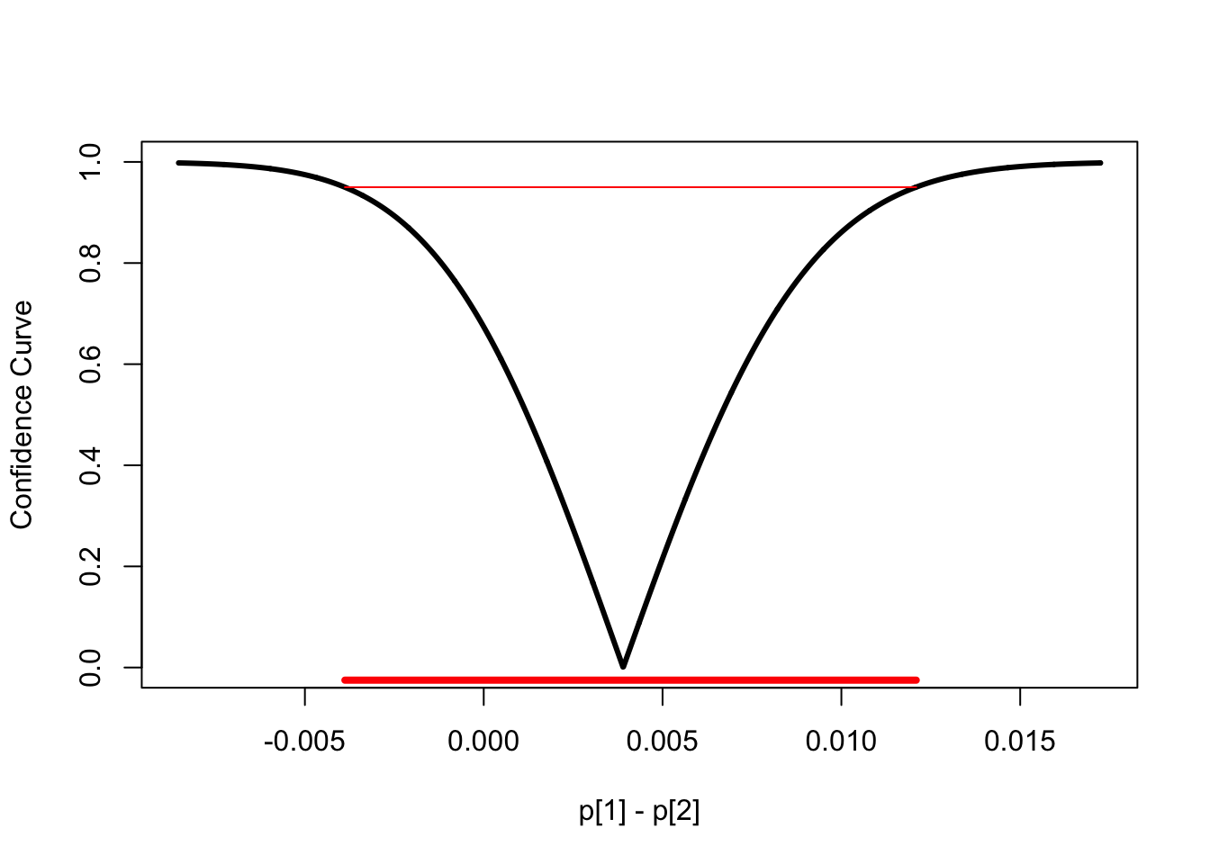
But why stop with a 95% confidence interval? We can show all possible confidence intervals for \(\delta\) via the confidence curve by calling plot.cconf():
plot.cconf(conf.diff.props,
           xlab = 'p[1] - p[2]')
Yes, \(\delta = 0\) (no difference) is contained in the 95% confidence interval, so we would fail to reject \(\delta = 0\) at a 5% significance level. But the weight of the evidence is for the mask-PSA intervention being more effective than no-intervention. We can make this clearer by plotting the confidence density for \(\delta\):
plot.dconf(conf.diff.props,
           xlab = 'p[1] - p[2]')

x.shade <- seq(0, 0.03, length.out = 100)
polygon(x = c(0,
              x.shade,
              rev(x.shade),
              0),
        y = c(0,
              rep(0, length(x.shade)),
              conf.diff.props$dconf(rev(x.shade)),
              0),
        col = rgb(0, 1, 0, alpha = 0.5))
The green shaded area is the fiducial probability associated with \(\delta\) being positive (positive impact of the mask-PSA), which we can compute using the complementary confidence distribution:
1-conf.diff.props$pconf(0)## [1] 0.836919483.7% of the evidence is in favor of the mask-PSA having some positive impact compared to no-PSA. This corresponds to the \(P\)- value for the left-sided test \[\begin{aligned} H_{0} &: \delta \geq 0 \\ H_{1} &: \delta < 0 \end{aligned}\] We get the \(P\)-value for the right-sided test \[\begin{aligned} H_{0} &: \delta \leq 0 \\ H_{1} &: \delta > 0 \end{aligned}\] by direct use of the confidence distribution:
conf.diff.props$pconf(0)## [1] 0.1630806and thus have weaker evidence for the mask-PSA being less effective than the no-PSA intervention.
The main takeaway from this study, of course, is that we just don’t know for sure whether the mask-PSA worked or not. The weight of evidence is in favor of the mask-PSA working, but we would need a new study, with more participants, to get a better idea. Though, since we can never step in the same river twice, other things are clearly different in Denmark now compared to April and May of 2020. This reminds us that there is no “the effect of a mask-PSA,” as the effectiveness of that PSA will vary depending on all of the contingencies currently in play.
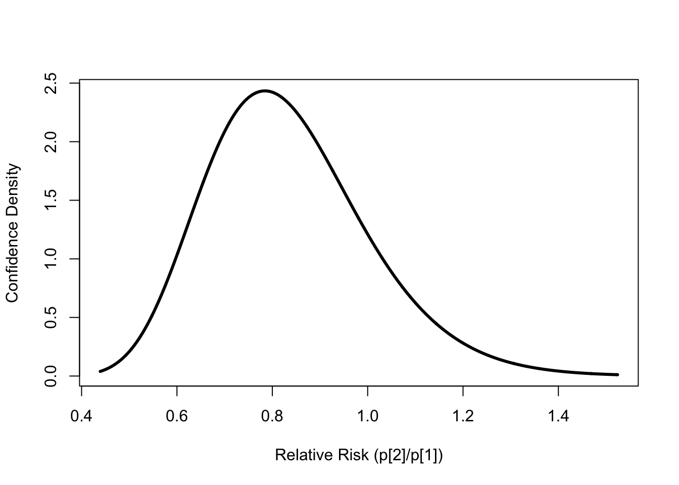
We can repeat the same analysis with the relative risk and odds ratio, other common parameters when assessing changes in risk. The relative risk (or risk ratio) is defined as
\[\begin{aligned} \rho &= \frac{\text{Risk in Treatment}}{\text{Risk in Control}} \\ &= \frac{p_{T}}{p_{C}} \end{aligned}\]
and we can compute the confidence functions using clp’s riskratio.conf().
conf.rel.risk <- clp::riskratio.conf(x, n)

and get out the median of the confidence distribution
conf.rel.risk$qconf(0.5)## [1] 0.8182709which matches the obvious point estimate of the relative risk from the sample:
p[2]/p[1]## [1] 0.8182937We compute a 95% confidence distribution for \(\rho\) using the confidence quantile:
conf.rel.risk$qconf(c(0.025, 0.975))## [1] 0.5493596 1.2186575So the data are consistent with anywhere from a 45% reduction in risk for the treatment group to a 22% increase in risk for the treatment group. This matches the portion of their results synopsis:
Although the difference observed was not statistically significant, the 95% CIs are compatible with a 46% reduction to a 23% increase in infection.
Though, again, they’re presumably using a Wald statistic rather than a score statistic to compute their confidence interval.
The \(P\)-value for a two-sided test of \(\rho = 1\) (if we must have it), is
conf.rel.risk$pcurve(1)## [1] 0.3261612where we use \(\rho = 1\) since a risk ratio of 1 indicates no difference in risk between the two groups. This exactly matches the \(P\)-value for \(\delta = 0\).
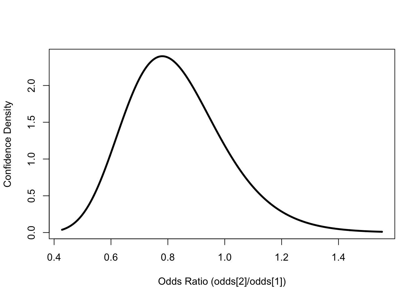
Finally, all the same analyses, but using the odds ratio \[\begin{aligned} \omega &= \frac{\text{Odds(Infection; Treatment)}}{\text{Odds(Infection; Control)}} \\ &= \frac{p_{T}/(1 - p_{T})}{p_{C}/(1-p_{C})} \end{aligned}\] I’ll leave out the color commentary this time:
conf.odds.ratio <- clp::oddsratio.conf(x, n)

conf.odds.ratio$qconf(0.5)## [1] 0.8150468odds.control <- p[1]/(1-p[1])
odds.treatment <- p[2]/(1-p[2])
odds.treatment/odds.control## [1] 0.8150462conf.odds.ratio$qconf(c(0.025, 0.975))## [1] 0.541522 1.226716conf.odds.ratio$pcurve(1)## [1] 0.3269062