Bounded Bayes: Markov Chain Monte Carlo (MCMC) for Posteriors of Bounded Parameters

This is largely a note to my past-self on how to easily use Markov Chain Monte Carlo (MCMC) methods for Bayesian inference when the parameter you are interested in has bounded support. The most basic MCMC methods involve using additive noise to get new draws, which can cause problems if that kicks you out of the parameter space.

Suggestions abound to use the transformation trick on a bounded parameter \(\theta\), and then make draws of the transformed parameter. But I could not easily find a worked example. So here’s that worked example.

Suppose we want to simulate from the posterior distribution of a parameter \(\theta\) with a bounded parameter space. Select an invertible function \(g\) that maps the bounded parameter space to the real line, i.e. \[\psi = g(\theta) \text{ where } g : \Theta \to \mathbb{R}.\] Then simulate from the posterior density \(f_{\Psi \mid \mathbf{X}}(\psi \mid \mathbf{x})\) in terms of the transformed parameter \(\psi\). By the transformation theorem, \[\psi \mid \mathbf{X} = \mathbf{x} \sim f_{\Psi \mid \mathbf{X}}(\psi \mid \mathbf{x}) = \frac{f_{\Theta \mid \mathbf{X}}(g^{-1}(\psi) \mid \mathbf{x})}{|g'(g^{-1}(\psi))|},\] where the posterior \(f_{\Theta \mid \mathbf{X}}\) is known, at least up to the likelihood and prior.

Let’s use this to simulate a success probability for a binomial proportion from the posterior density \(f_{P \mid X}(p \mid x)\). Here, because \(p \in (0, 1)\), it’s natural to use the logit function to map from \((0, 1)\) to \((-\infty, \infty)\): \[ \psi = \operatorname{logit}(p) = \log \frac{p}{1-p} \] The transformation theorem then gives the posterior in terms of \(\psi\) as: \[ \begin{aligned} f_{\Psi \mid X}(\psi \mid x) &= \frac{f_{P \mid X}(\operatorname{logit}^{-1}(\psi) \mid x)}{|\operatorname{logit}'(\operatorname{logit}^{-1}(\psi))|} \\ &= f_{P \mid X}(p \mid x) \times p(1-p) \end{aligned} \] where \[ p = \operatorname{logit}^{-1}(\psi) = \frac{e^{\psi}}{1 + e^{\psi}}. \] Sampling \(\psi\) via a random walk and using the Metropolis-Hastings update rule now gives a chain in terms of \(\psi_{1}, \psi_{2}, \ldots, \psi_{B}\), which can be transformed via \(\operatorname{logit}^{-1}\) into a chain in terms of \(p_{1}, p_{2}, \ldots, p_{B}\).

Let’s use the Jeffreys prior for \(P\): \(P \sim \operatorname{Be}(1/2, 1/2)\). In this case, we can easily work out the posterior, but let’s use a lookup table put together by Ruoyong Yang and Jim Berger. The posterior distribution of \(P\) given we observe \(x\) successes in \(n\) trials is \(P \mid X = x \sim \operatorname{Be}(x + 1/2, n - x + 1/2)\).

We know the posterior in terms of \(\psi = \operatorname{logit}(p)\) is \[f(\psi \mid x) \propto f(x \mid \psi) f(\psi).\] Moreover, the posterior in terms of \(p\) is

\[ \begin{aligned} f(p \mid x) &\propto f(x \mid p) f(p) \\ &= \texttt{dbinom(x, n, p)*dbeta(p, 1/2, 1/2)} \end{aligned} \] And the posterior in terms of \(\psi\) is just the posterior in terms of \(p\), modified by the multiplicative factor that takes care of the transformation from \(p\) to \(\psi\) \[ f(\psi \mid x) \propto f(p \mid x) p (1-p) \bigg\rvert_{p = \operatorname{logit}^{-1}(\psi)} \] This is the posterior distribution we will make draws from using Metropolis-Hastings, i.e. given that we have \(\psi_{1}, \psi_{2}, \ldots, \psi_{t-1}\), generate a new potential draw \(\psi_{t} = \psi_{t-1} + \epsilon_{t}\) where \(\epsilon_{t} \sim N(0, \sigma^{2})\), and compute \[ A = \min \left\{1, \frac{f(\psi_{t} \mid x)}{f(\psi_{t-1} \mid x)} \right\}. \] We then accept \(\psi_{t}\) with probability \(A\), or otherwise repeat the previous draw, i.e. \(\psi_{t} = \psi_{t-1}\).

Let’s define some functions for the logit and inverse logit functions:

logit <- function(p) log(p/(1-p))
invlogit <- function(psi) exp(psi)/(1 + exp(psi))

And to compute the numerator of the posterior distribution of \(\Psi \mid X = x\):

posterior.numer <- function(psi){
  p = invlogit(psi)
  dbinom(x, n, p)*dbeta(p, 1/2, 1/2)*p*(1-p)
}

Now we’re ready to simulate from the posterior distribution via Metropolis-Hastings:

set.seed(1) # For reproducibility

n <- 2
x <- 1

B <- 100000

psis <- rep(0, length(B))

for (b in 2:B){
  candidate.psi <- psis[b-1] + rnorm(1, 0, 1)
  
  A <- min(c(1, posterior.numer(candidate.psi)/posterior.numer(psis[b-1])))
  
  if (runif(1) <= A){ # Accept candidate.psi with probability A
    psis[b] <- candidate.psi
  }else{ # Reject candidate.psi and repeat psis[b-1]
    psis[b] <- psis[b-1]
  }
}

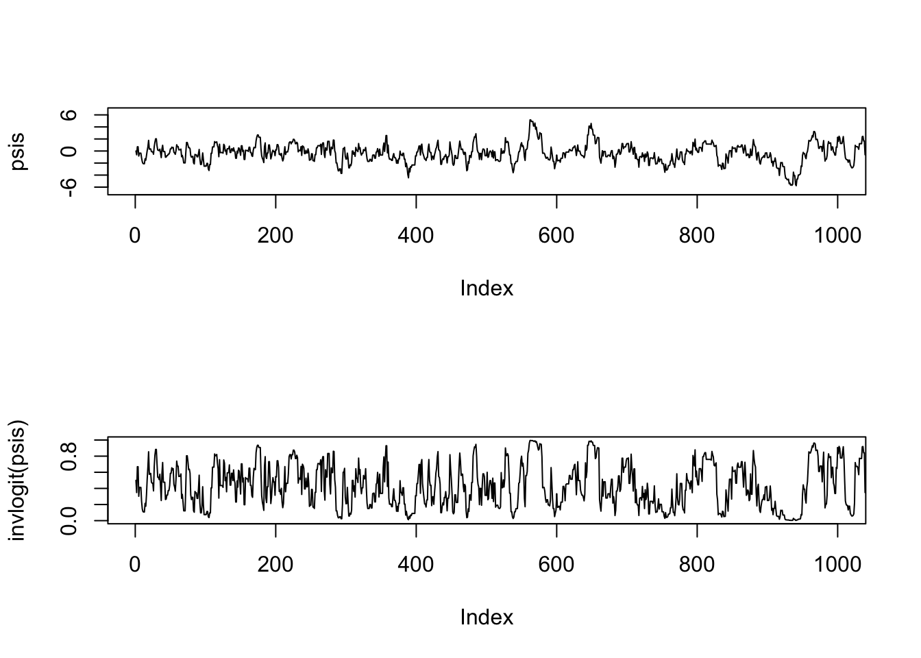
We can view the Markov chains for the posterior distributions in terms of either the \(\psi\)s or the \(p\)s:

par(mfrow = c(2, 1))
plot(psis, type = 'l', xlim = c(1, 1000))
plot(invlogit(psis), type = 'l', xlim = c(1, 1000))

And the posterior distributions in terms of either the \(\psi\)s or the \(p\)s:

par(mfrow = c(1, 2))
hist(psis, breaks = 'FD', main = '')
hist(invlogit(psis), breaks = 'FD', freq = FALSE, xlim = c(0, 1), main = '')
curve(dbeta(p, x + 0.5, n - x + 0.5), xname = 'p', add = TRUE, col = 'blue')

Clearly, the simulated draws match the true posterior, as they must.

• statistics
• reminders
• worked examples